
Population dynamics of one species
Basic model of population dynamics
generation/time
Let's start with the jellyfish story at the beginning and gradually move on to the basic model of population dynamics. The jellyfish went from one individual to two individuals in the first division.
In fact, this is not "one individual divided and increased by another'', but rather "two individuals germinated within one individual's body, and as a result, the original individual died”. Many species of jellyfish have a polyp stage that lives a benthic life and reproduces asexually, and a Medusa stage that lives a planktonic life and reproduces sexually. (However, Rathkea octopunctata reproduces asexually during the Medusa stage.) There's a lot more to the life cycle of a jellyfish in the real world, but for the sake of simplicity, let's think of Rathkea octopunctata as splitting and changing generations.
The fact that the next day after splitting into 2 individuals resulted in 4 individuals is the result of the division of each 2 individuals from the 2 individuals of the 2nd generation as the 3rd generation. Here, generation is called time, and this is represented by t. The number of individuals at time t is called Nt. Now, let's express this change in the number of individuals with a formula.
Number of individuals N0 = 1 at t = 0, they split and at t = 1 N1 = 2. Considering that the original individual died and the number of individuals decreased, this can be represented by a formula as follows.
N1 = N0 + (increased population) – (decreased population) = 1 + 2 – 1 = 2
The number of individuals at t = 2 can also be considered in the same way. The number of individuals that increased and the number of individuals that decreased were expressed using N1 as follows.
N2 = N1 + 2 x N1 – 1 x N1 = 2N1
A series of cycles until a child born at a certain time gives birth to the next. For organisms whose life cycles, a series of cycles until a child born at a certain time gives birth to the next, are synchronized in all individuals in the population and whose generations do not overlap, this sequential calculation can predict future population numbers. Let's generalize and express this. The population change of the generation at time t and the next generation at time t + 1 can be expressed as follows.
Nt + 1 = Nt + b Nt – d Nt
where b is the rate of increase per unit time and d is the rate of decrease per unit time. Summarizing the right side of this equation with Nt ,
Nt + 1 = (1 + b – d) Nt
Furthermore, if the difference b – d between the rate of increase and the rate of decrease is summed up as the net rate of increase R, it can be expressed as
Nt + 1 = (1 + R) Nt (6.1)
This time, the relationship between N2 and N0 can be expressed as a formula as follows.
N2 = (1 + R) N1 = (1+R) (1 + R) N0 = (1 + R)2 N0
Generalizing this formula, the number of individuals in the generation at time t can be expressed by the number of individuals N0 and R at time 0 as follows.
Nt = (1 + R)t N0 (6.2)
 This is the most basic model of population dynamics. In fact, the initial calculation is
N30 = 230 x 1
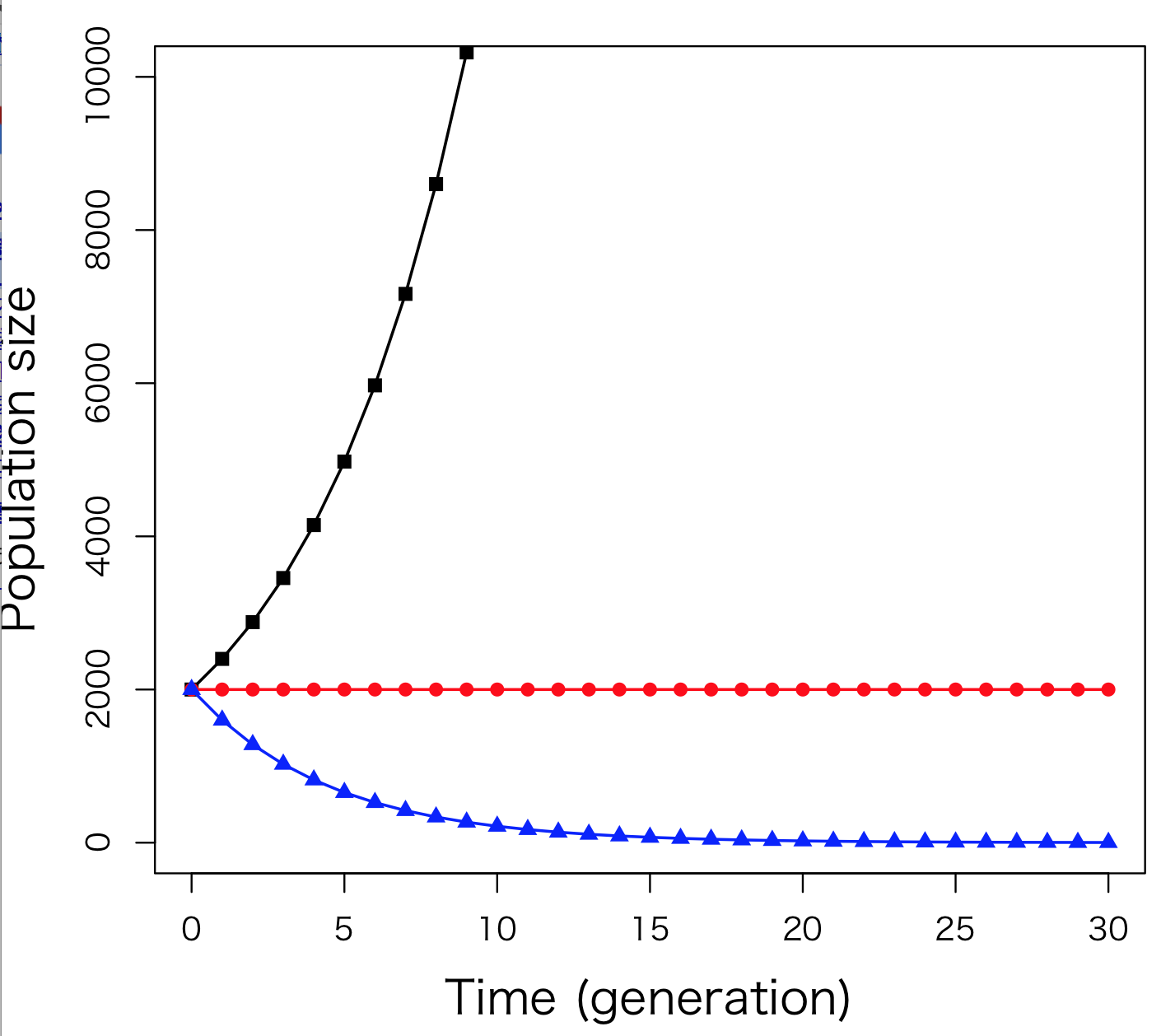
Equation 6.2 can be thought of as a relational expression between Nt and N0, or between Nt and R, but here we think of it as a relational expression between the number of individuals Nt and time t. In other words, this formula expresses time-varying population size, that is, population dynamics. Let's plot the relationship between Nt and t with N0 = 2000 (right figure). When R takes a positive value (black polygonal line, R = 0.2), the slope becomes steeper as the number of individuals Nt increases, and the number of individuals that proliferate by the next hour increases. On the other hand, when R takes a negative value, the population size decreases (blue line, R = –0.2), and when R = 0, the population size does not change (red line).
internal natural increase rate
In Rathkea octopunctata story earlier, the scenario was that "the generations do not overlap". However, since Rathkea octopunctata actually splits between day and night, the generations overlap.Since the breeding timing of each parent is different, there are large parent individuals and small size individuals at the same time. Therefore, multiple generations are mixed at the same time. In order to accurately predict population dynamics in such cases of non-synchronized breeding and overlapping generations, shorter time units are better. When the unit of time is shortened to the limit, the population growth rate (dN/dt) at time t is expressed by the following differential equation.
\( \frac{dN}{dt} = rN \) (6.3) 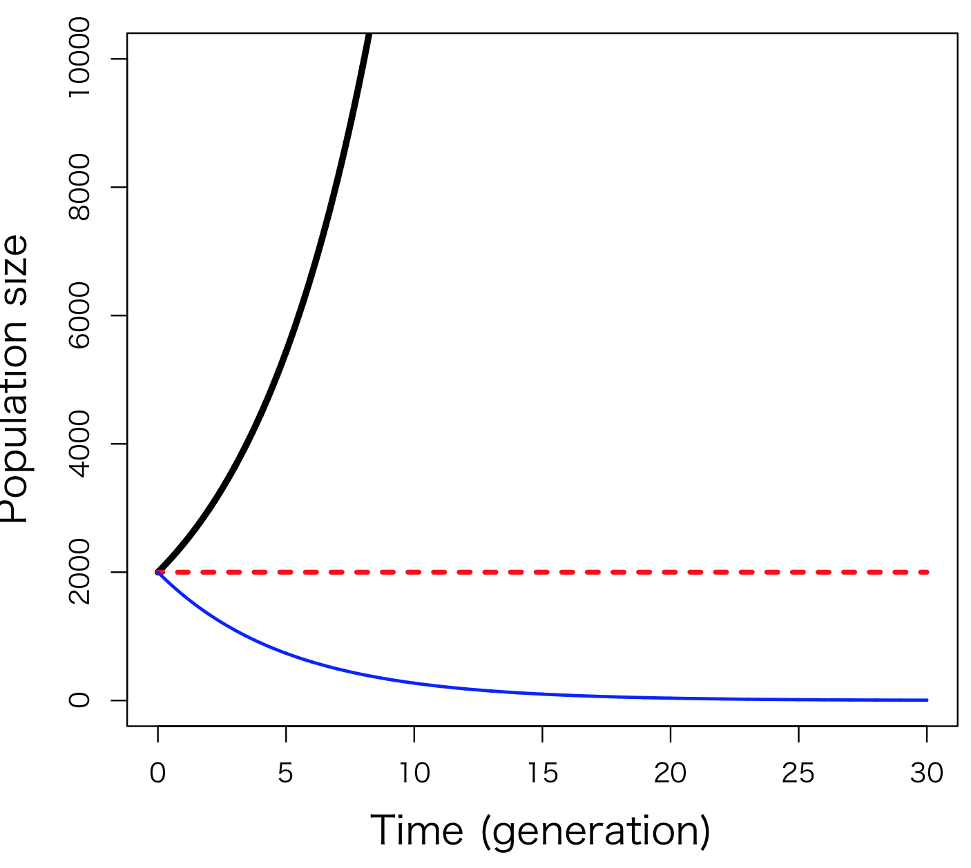
This is the differential equation version of Equation 6.2. dN/dt is the “slope” at a point in time of a curve showing how population changes over time. Also, in this formula, r is the differential equation version of R that appeared in formula 6.1, and is the value obtained by subtracting the instantaneous death rate from the instantaneous birth rate per individual. r is named the internal natural increase rate. The population dynamics expressed by Equation 6.3 are also very similar to those of Equation 6.2 (Fig. 6-2B) and if r > 0 the population will increase, if r < 0 it will decrease, and if r = 0, the population will not change.
So far, the number of individuals increases exponentially as long as r > 0. In other words, many of the possible factors of real population dynamics that would limit population growth are not yet included. From the next section onwards, I will list the factors that suppress population growth, with a particular focus on intraspecific and interspecific relationships.
Density effect/carrying capacity
In order for organisms to grow and produce offspring, they must acquire resources such as food, habitat, and mates. However, resources are finite, and some resources vary greatly in quality.
While the population is small, it is easy to acquire resources and can choose good resources, so the population growth rate will be high.
On the other hand, if the number of individuals increases, the population as a whole will run out of resources, and it is expected that the growth rate, survival rate, and reproductive power (number of eggs laid) of individuals will decline, and the growth rate of the population will also decline. When the population size reaches a certain number of individuals, the growth rate should be 0, and when the number of individuals increases further, the growth rate should be negative. This is also based on the premise that the distribution area of the individuals that make up the population does not change greatly according to the number of individuals, that is, the density increases as the number of individuals increases. The phenomenon that the growth rate decreases as the density increases is called the density effect. However, population growth rates are not necessarily higher at lower densities.If the density is too low, it may not be possible to find a mate and leave offspring. In addition, by living in groups, stress such as dehydration can be alleviated, and defense effects against predators can be obtained. Under these circumstances, the higher the density, the higher the growth rate. This phenomenon is called the Ally effect.
Let's improve the differential equation 6.3 above to express the density effect. First, the number of individuals when the number of individuals increases and the growth rate becomes 0 is defined as a constant K. In this case, K is called the environmental carrying capacity. Where food or habitat is abundant, K is large, and where food or habitat is scarce, K is small. When the number of individuals N becomes K, we can use a formula that dN/dt = 0, so we should multiply formula 6.3 by the term (K – N). But rN (K – N) is in trouble. (K – N) is close to K when N is small.Then, when N is small, the value of rN (K – N) becomes very large compared to rN. Therefore, the following equation is obtained by multiplying Equation 6.3 by the term obtained by dividing (K – N) by K.
\( \frac{dN}{dt} = rN \frac{K - N}{K} \) (6.4)
In the model of formula 6.4, (K – N)/K takes a value close to 1 while the number of individuals is small, so it shows a proliferation rate close to that of formula 6.3. However, when N increases, (K – N)/K approaches 0, so the proliferation rate dN/dt decreases, and when N = K, the proliferation rate becomes 0. Therefore, when the initial population is small, the population dynamics are sigmoidal, as shown by the black curve in Figure 6.2D. Such an S-shaped curve is called a logistic curve. Of course, if the initial number of individuals is large, the curve will be a discontinuous S-shaped curve, and if the initial number of individuals exceeds K, (K – N)/K becomes negative, so the population size decreases, and the growth rate becomes 0 when N = K.
Also note that if we plot Equation 6.4 with dN/dt on the Y axis and the number of individuals N on the X axis, it becomes a negative quadratic function. When N is 0 or K, dN/dt = 0, and when 0.5K, dN/dt reaches its maximum value. In the range where N is greater than 0 and less than K, dN/dt is positive and the population increases. On the other hand, when N exceeds K, dN/dt becomes negative and the population decreases. If the population is not 0, the population of this population will eventually stabilize at K. In this way, by drawing differential equations, we can know the conditions under which the population increases, the conditions under which it decreases, and the conditions under which it stabilizes at a constant number.
Equation 6.4 is the underlying model for many complex demographic models. However, equation 6.4 is still too simplistic to represent real population dynamics. In fact, equation 6.4 requires (1) no change in environmental conditions and resources, (2) no variation in the traits of individuals that make up the population, (3) no immigration and no evolution of individuals, (4) the density effect acts in response to population fluctuations without a time lag, and (5) there is no interspecies relationship. In reality, environmental conditions such as temperature fluctuate, and the population of organisms that feed on them also fluctuates. Furthermore, for example, the lack of food due to high density will appear as changes in growth rate and egg production after a short time has passed since the high density. There is a time lag in the maritime density effect. Section 6-2 introduces a model that assumes interspecies competition and predator-prey relationships.
As a simple model that assumes a situation slightly different from equation 6.4, let's incorporate the density effect into the non-overlapping population dynamics model (Equation 6.1) introduced at the beginning. First, rewrite equation 6.1 as follows.
Nt + 1 = Nt + Nt R (6.1)
Here, multiplying the population net increase rate R by the density effect (K – N)/K as in equation 6.4 yields the following equation.
\( N_{t + 1} = N_t + N_tR \frac{K - N_t}{K} \) (6.5)
Interestingly, the population dynamics of Equation 6.5 are not straightforward. Similar to Equation 6.4, it may result in population convergence to carrying capacity K (Figure 6-2C), but this only happens when R is small. If R is large, the population increases too much and exceeds K, and the next time the population decreases too much and falls below K (Fig. 6-4). When we put in various values of R, we can see that the pattern of population dynamics changes according to R like the number of individuals converges to K with damped oscillation (Fig. 6-4A), a two-point cycle in which two populations alternate (Fig. 6-4B), a four-point cycle (Fig. 6-4C), or Chaos where population dynamics change greatly due to small differences in initial values (Fig. 6-4D). In other words, even if the abiotic environmental conditions were perfectly stable and there were no influences from other species, the mere density effect and high growth rate would destabilize population dynamics and sometimes lead to extinction. (Extinctions are occurring in the simulation in Figure 6-4D).