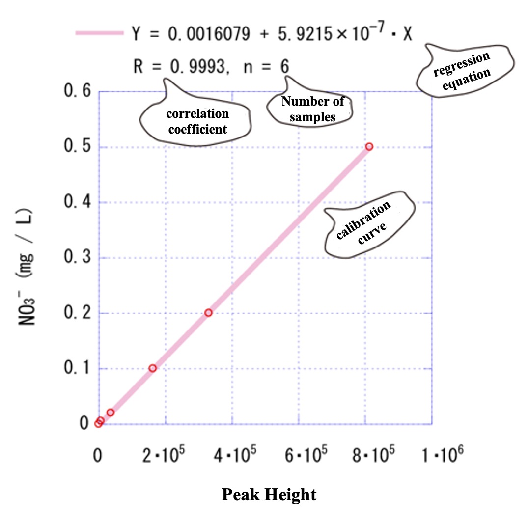
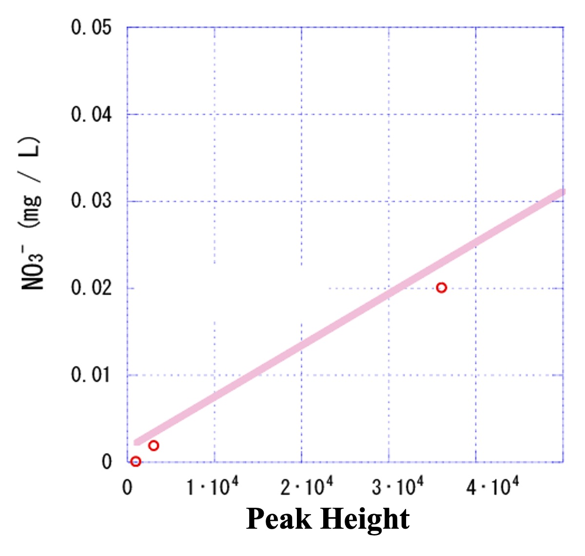
The plot of Example 1-1) is shown again.

The low concentrations near the origin also appear to be on the calibration curve.
Expand the low-concentration range.

Before the expansion, all plots appeared to be on the calibration curve. However, when the low concentration range was expanded, it was found that the low concentration plots deviated slightly from the calibration curve.
In such a case, substituting the signal intensity (peak height) of the unknown sample at low concentration into the regression equation of the previous calibration curve to obtain the concentration will result in a large error. It is necessary to consider the reason why this plot does not ride on the calibration curve.
① Is it due to an accidental error?
② Is it not a coincidence that it deviates from the calibration curve in the same way no matter how many times it is measured?
Let us consider it in two ways.
Let's address this first, starting with ②.
One way to solve the problem of (2) is to create a calibration curve that also covers a low concentration range. Even though it may not be on a straight calibration curve, if the reliability of the measurement is confirmed, such a method may be used. For example, you can use two different calibration curves, one made with only standard samples in the low concentration range and the other made with standard samples in the high concentration range. Or, if the plots of the low and high concentration ranges can be approximated by a single quadratic curve (or exponential curve), you can use that curve to create the calibration curve. To convert the curve into a formula, plot it on an Excel chart and use the approximate curve function.
Notes: Note that in the case of curve approximations, small deviations can lead to large errors. You must make sure that the concentration of the unknown sample falls within the concentration range of the standard sample. Remember to make sure that the plot of the standard sample is on the approximation curve displayed in Excel. Often, it will be plotted in a totally different place, or worse, the top of the quadratic curve will fall within the quantitation range of the calibration curve.
① is the issue of "tolerance for chance error," or in other words, the control of measurement accuracy. Measurement accuracy is the degree of variation (standard deviation) after repeated measurements. The error is expressed as how much percentage of that variation is tolerated relative to the mean value.
Below are examples of standard deviation and error calculations.
For measurement item x, a repeated analysis was performed i times. The average, variance, standard deviation, and error are calculated as follows.
Mean (ave) :1/n×Σxi (Σは、i=1~nの積算)
Variance (S) :1/(n-1)×Σ(xi – ave)2
Standard deviation(σ) :S0.5
Standard error :σ/ave
Standard error (%) :(σ/ave)×100
You don't have to remember about variance and standard deviation, as they are built into the function calculator and Excel functions. Still, let's review the calculation method just in case. Please note the values in the blanks for variance S and standard deviation σ below.
Results of repeated measurements:20, 21, 20, 19, 20, 18, 21, 20, 19, 22
ave = 20、 S = 、σ = 、Standard error = 5.77 %
The results of the above measurement, simply multiplied by 10, are shown below.
Results of repeated measurements (B):200, 210, 200, 190, 200, 180, 210, 200,
190, 220
ave = 200、 S = 、σ = 、Standard error = 5.77 %
Comparing the previous results
amplified by a factor of 10, ave is 10 times greater, S is 100 times greater, and σ is 10 times greater. The standard errors are the same for (A) and (B). Now you have some idea of what standard error means.
In analytical chemistry, signal intensity is sometimes amplified to increase measurement sensitivity. This is the same as using an amplifier to amplify the volume of a speaker. However, if the signal (voice) and noise are amplified together, the audibility (measurement accuracy: error) will not change.
Now, let us return to ①, "Tolerance for chance errors". The analyst determines what percentage of standard error is acceptable. For example, if the standard error of 10% or less is defined as valid, the results of (A) and (B) are considered valid. However, do not forget to note the number of repeat measurements (n). It is not realistic to repeat the measurement 10 times each time for an unknown sample, so we often measure a standard sample 10 times to guarantee the accuracy of the analysis. It is important to note that the analysis results will vary widely (accuracy will deteriorate) in the low and high concentration ranges. If you want to guarantee the measurement accuracy of an unknown sample at a low or high concentration, you will need to perform repeated measurements of a standard sample close to that concentration to check for errors.
After explaining the lower and upper limits of quantification on the next page, you will be asked to work through the exercises.
Note that the fact that the plot of the standard sample is approximated by a curve suggests that some analytical problem has occurred. The reason for this should be considered and addressed to improve analytical techniques.